class: center, middle .header[ <small>Created with [remark](https://github.com/gnab/remark)</small> ] # AI Bytes ## Classification <hr> Dileep Patchigolla May 5, 2020 --- # About me <br><br> .center.h1[Dileep Patchigolla] <br><br> - Lead Engineer @ Search - With Target since July 2018 - MS, Computational Data Analytics - Georgia Tech - B.Tech, Mechanical Engineering - IIT Madras --- # Agenda - What is Classification? - Statistical approach: Logistic Regression - Geometric approach: SVM - Rules based approach: Decision Trees - Rules based approach, combining models (ensemble): Random Forest --- ## Classification Binary classification: _Yes / No Problems_ - Should a credit card application be approved? - Is this transaction genuine? - Does the mail belong to spam? - Is this customer male or female? <br> <br> <br> -- _But what if there are more than two classes?_ Multi-class classification: - What marketing campaign should I send to a customer? - Which category does a query belong to? - Who is the person in an image? --- ## IRIS Dataset - Features - Sepal length & width, Petal length & width - Label - Setosa, Versicolor, Virginica .center.image-50[] -- <br> ### Binary Classification: - Let's consider two classes: Versicolor and Virginica -- - Call one class as 0 and other as 1. Typically based on which case we consider as _positive_. Here the choice is arbitrary - Come up with a function `$f(x)$` which gives the value of `$y$`, for a given `$x$` --- class: center, middle # Logistic Regression --- # Linear Regression - Quick Review .center.image-50[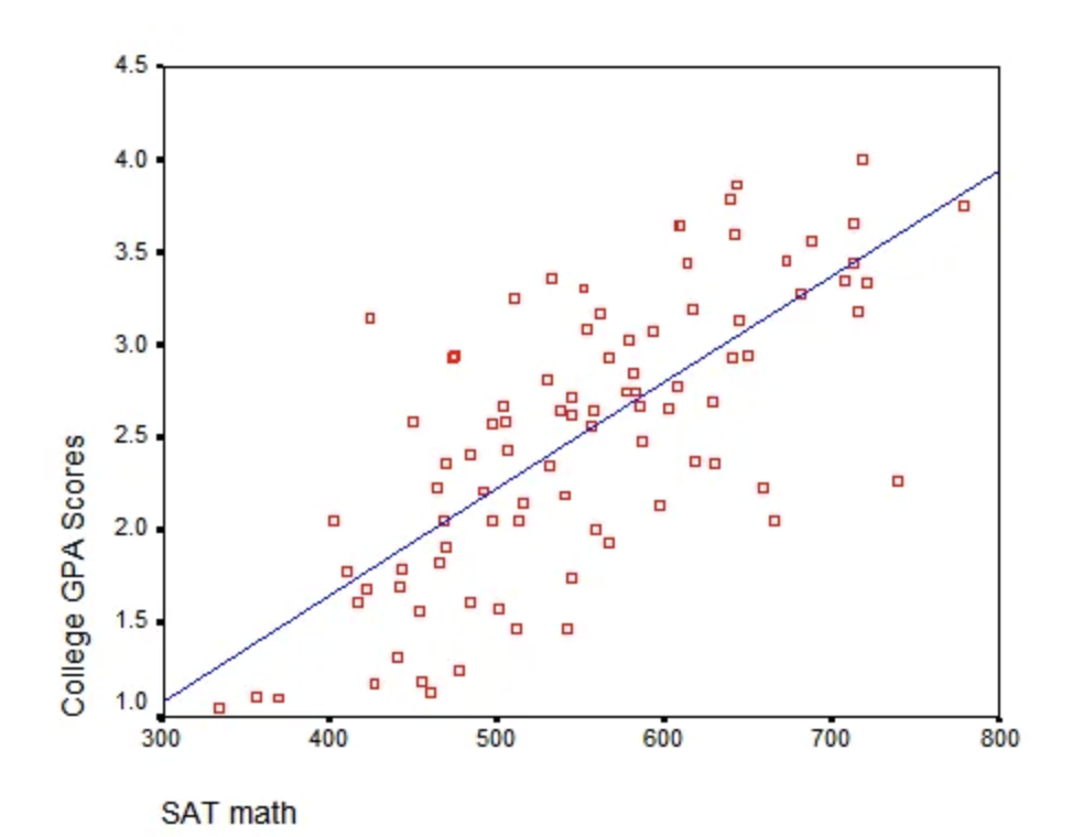] <br> `$\qquad\qquad\qquad\qquad\qquad\qquad y = w_{0} + w_{1} x_{1}$` - `$y$` is continuous and its range can be very wide. - Fit a straight line on the features, to get an estimate of `$y$` --- # Logistic Regression `$f(x) = w_0 + w_{1}x_{1}$` - Similar to Linear Regression (linear formulation) - But `$y$` is not continuous. Takes only two values, 0 and 1 -- - Make discrete problem to continuous problem. Predict `$P(Y==1|X)$`, i.e., _probability_ of `$y=1$` -- - Need some translation that always binds `$f(x)$` between 0 and 1 --- # Sigmoid function `$P(Y==1|X) = \frac{1}{1+ e^{-f(x)}} = \sigma(f(x))$` .center.image-50[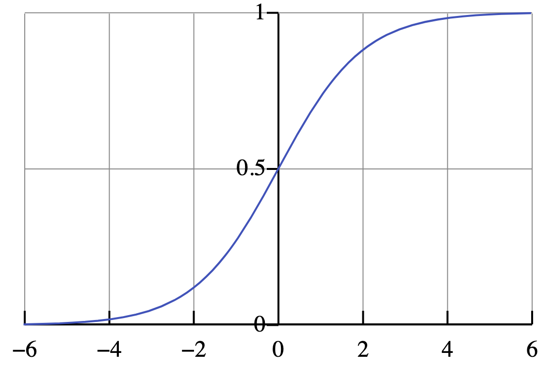] - Bounded between 0 and 1 - Asymptotically gets closer to 0 and 1 --- # Logit function - So what does the linear equation `$f(x)$` mean? -- Lets denote `$P(Y==1|X)$` by `$p$` `$\qquad\qquad\qquad p = \frac{1}{1+ e^{-f(x)}}$` -- `$\qquad\qquad\qquad \frac{1}{p} = 1+ e^{-f(x)}$` -- `$\qquad\qquad\qquad \frac{1-p}{p} = e^{-f(x)}$` -- `$\qquad\qquad\qquad \frac{p}{1-p} = e^{f(x)}$` -- `$\qquad\qquad\qquad log(\frac{p}{1-p}) = f(x)$` - `$log(\frac{p}{1-p})$` is called logit function - log-odds ratio - odds = `$\frac{\text{#yes}}{\text{#no}}$` --- # Weights - `$f(x)$` can take several variables. i.e., `$f(x) = w_0 + w_{1}x_{1} + . . . w_{m}x_{m}$` - In our example, `$x_{1} = $` Sepal length, `$x_{2} = $` Sepal width etc. - But what about `$w_{0}, w_{1},...w_{n}$`? - Use the available data and their labels. - Create a loss function and try to minimize that --- # Log Loss <br/><br/> `$ \qquad\qquad\qquad\qquad \hat{y} = P(Y==1|X) = \frac{1}{1+ e^{-(w_0 + w_{1}x_{1} + . . . w_{m}x_{m})}} $` <br/><br/> `$ \qquad\qquad\qquad \qquad L = -\frac{1}{n} \Sigma_{i=1}^{n} \enspace y_{i} log(\hat{y_{i}}) + (1-y_{i}) log(1-\hat{y_{i}})$` - a.k.a. Binary Cross Entropy. Minimize this value - If `$y_{i}$` = 0, first part of the loss is zero and second part is active. Loss = `$log(1-\hat{y}_{i})$` -- - If `$\hat{y}_{i}$` is close to 0 (_correct prediction_), then `$1-\hat{y}_{i}$` is close to 1 and `$log(1-\hat{y}_{i})$` gets close to 0. Overall loss is zero -- - If `$\hat{y}_{i}$` is close to 1 (_wrong prediction_), then `$1-\hat{y}_{i}$` is close to 0 and `$log(1-\hat{y}_{i})$` gets close to `$-\infty$`. Overall loss is zero -- - If y = 1, the roles reverse. Loss = `$log(\hat{y}_{i})$` --- # Gradient Descent - Initialize weights randomly - Iterate until convergence: - Compute the Loss - Compute Gradient, and update weights -- - Fun fact: - `$\frac{\partial L}{\partial w} = -\frac{1}{n}\Sigma_{i=1}^{n} x_{i}(y_{i} - \hat{y}_{i})$` - `$\frac{\partial \sigma(x)}{\partial x} = \sigma(x) * (1-\sigma(x))^{[1]}$` .footnote[ [1] https://math.stackexchange.com/questions/78575/derivative-of-sigmoid-function-sigma-x-frac11e-x ] --- # Example .center.image-50[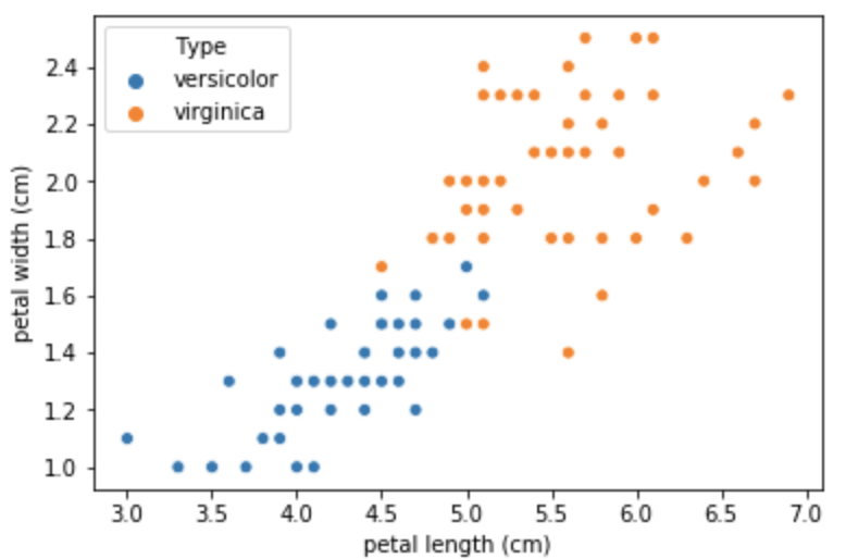] - `$x_{1}$` = petal length and `$x_{2}$` = petal width - y = 1 for versicolor and 0 for Virginica --- # Example (Cont.) logistic = LogisticRegression(solver="lbfgs") logistic.fit(iris_data.iloc[:, 2:4], iris_data["Y"]) print(np.round(logistic.intercept_,2)[0], np.round(logistic.coef_,2)[0]) - `$w_{0} = 17.55$`, `$w_{1}$` = -2.78, `$w_{2} = -2.39$` -- - `$\hat{y} = \frac{1}{1+ e^{-(w_0 + w_{1}x_{1} + w_{2}x_{2})}} $` -- - But `$\hat{y}$` is not 0 or 1. How do we convert `$\hat{y}$` to a yes/no decision? -- - Identify a threshold for cutoff .center.image-40[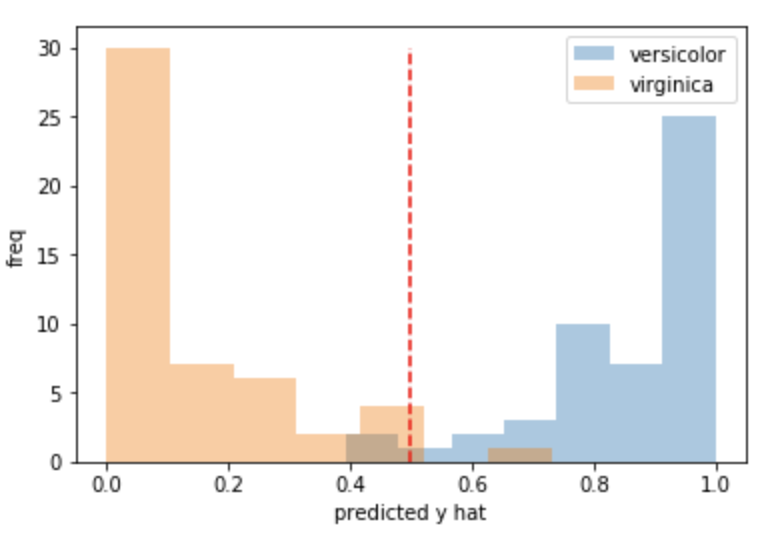] --- # Metrics For a given threshold: ### Confusion Matrix: .center.image-30[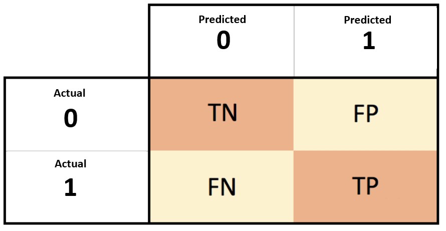] - Accuracy: `$\frac{\text{True Positive + True Negative}}{\text{Total Count}}$` - Precision: `$\frac{\text{True Positive}}{\text{True Positive + False Positive}}$` - Recall/True Positive Rate: `$\frac{\text{True Positive}}{\text{True Positive + False Negative}}$` - F1-Score: `$\frac{2}{Precision^{-1} + Recall^{-1}}$` - False Positive Rate: `$\frac{\text{False Positive}}{\text{False Positive + True Negative}}$` --- # Metrics For varying threshold: ROC Curve .center.image-40[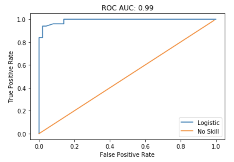] F1 Score at varying threshold .center.image-40[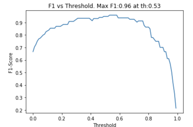] --- # Connection with Neural Nets <br><br><br> .center.middle.image-40[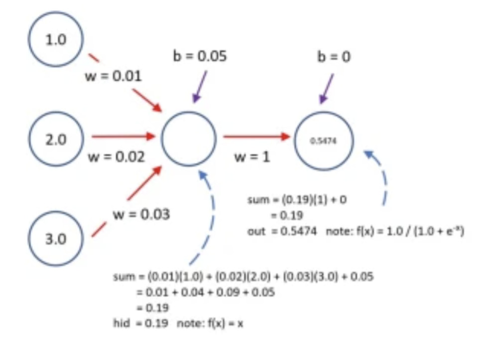] - Logistic Regression is a Neural Network with a single hidden layer, single unit, and sigmoid activation --- # Logistic Regression ### Pros - Very simple. Easy to train and interpret. One of the first models to try - Returns the probability of y = 1. Has more information than a simple yes/no prediction ### Cons - Can't learn a non-linear boundary - Forced to learn only additive interactions between the features - Suffers from convergence issues if complete separation exists For multi-class, can use multiple one-vs-rest models. --- layout: false class: center, middle # SVM --- # A Geometric Approach .center.image-50[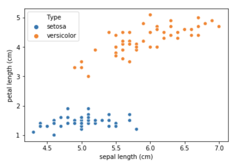] - How to separate them? --- # A Geometric Approach .center.image-50[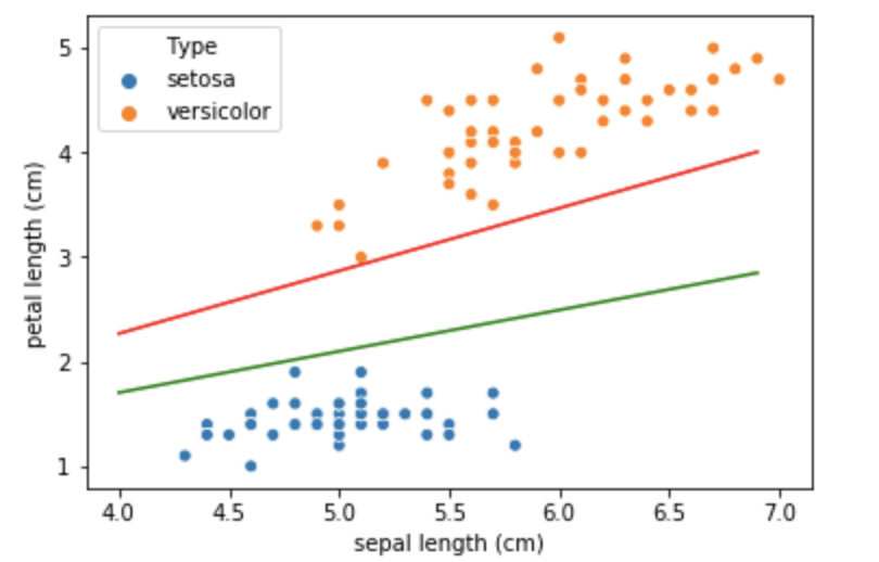] - Which line is better? --- # A Geometric Approach .center.image-50[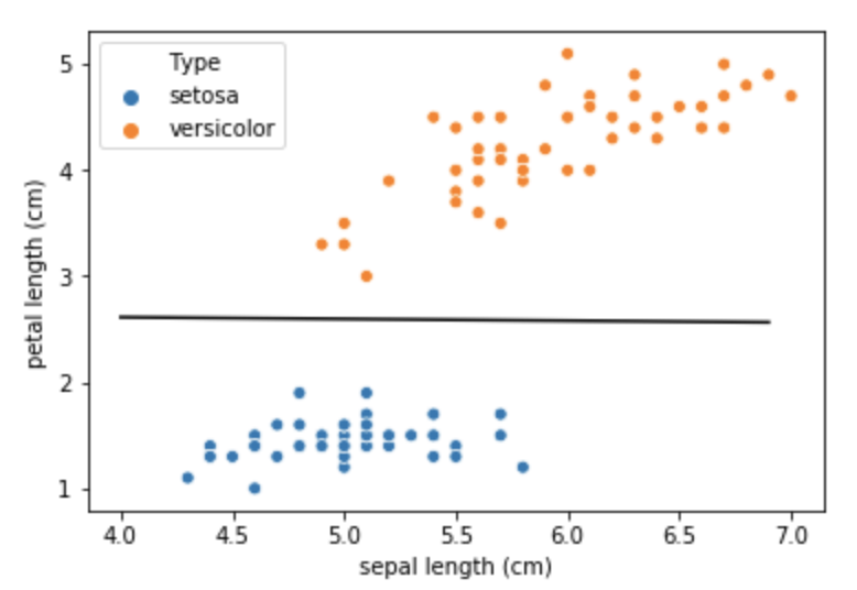] - How about this? --- # Maximum Margin Classifier Linearly separable data .center.image-40[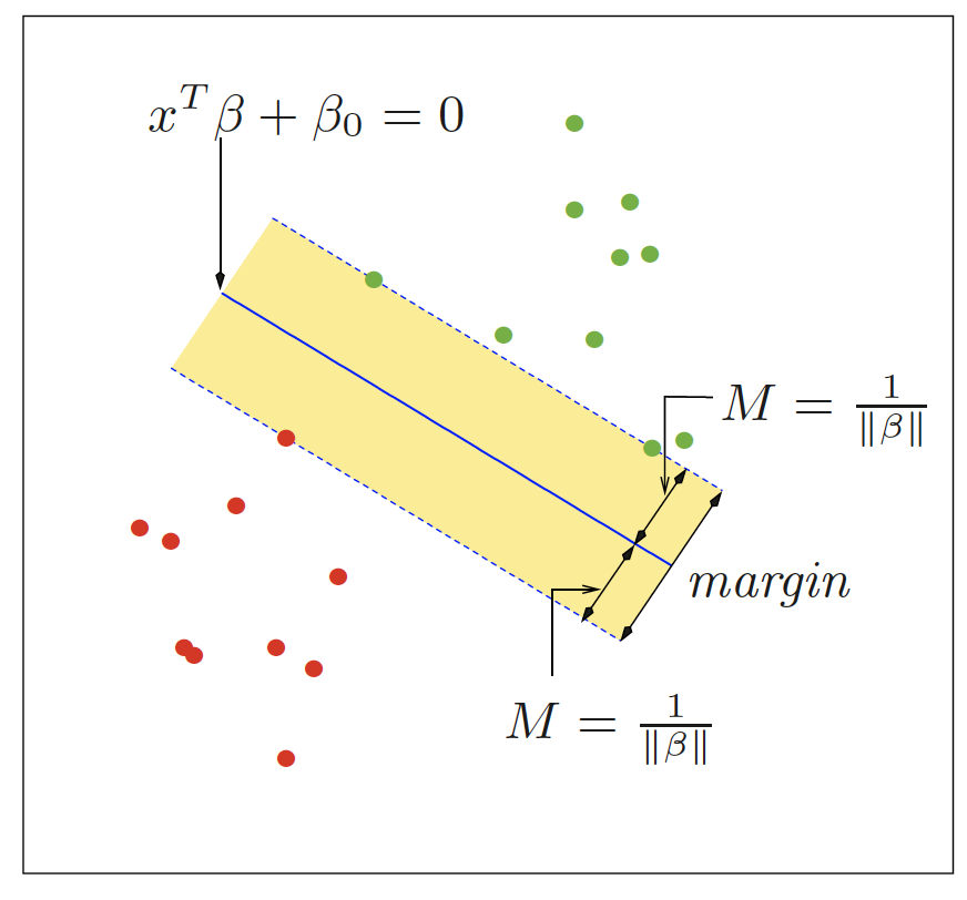] - Thick center line is called decision boundary - Both broken lines are equidistant to the decision boundary. The distance is called Margin (M) - Choose the center line such that M is maximum - Some points always touch the margin. These are called _support vectors_ --- # Maximum Margin Classifier Linearly separable data .center.image-40[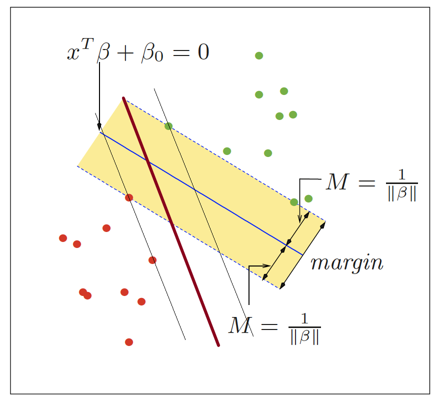] - The decision boundary can't tilt beyond this angle - Margin goes down --- # Maximum Margin Classifier Linearly separable data .center.image-40[] - The dotted lines take the form `$x^{T}\beta + \beta_{0} = 1$` and `$x^{T}\beta + \beta_{0} = -1$` - Dist. between parallel lines of form `$b_{0} + w_{1}x_{1} + w_{2}x_{2} = 0$` and `$b_{1} + w_{1}x_{1} + w_{2}x_{2} = 0$` is `$\frac{|b_{0} - b_{1}|}{\sqrt{w_{1}^{2} + w_{2}^{2}}}$` - Therefore, M = `$\frac{1}{||\beta||}$`. Maximize M = Minimize `$||\beta||$` --- # Maximum Margin Classifier <br> Objective Function: .center[Minimize `$||\beta||$`] s.t. `$\qquad\qquad\qquad\qquad\qquad y_{i} (x_{i}^{T}\beta + \beta_{0}) \geq 1 \quad \forall i=1,2,....N$` <br><br><br> - We denote `$y$` as +1/-1 - sign`$(x_{i}^{T}\beta + \beta_{0})$` = class of `$x_{i}$` for every `$i$` -- - So, what if the data is not separable linearly? --- # Support Vector Classifier Not separable linearly .center.image-40[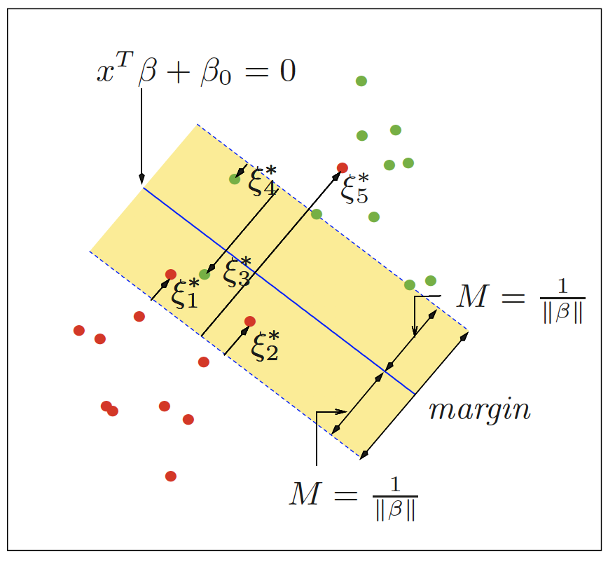] - An error term `$\xi$` is introduced. Measures distance from margin, to the wrong side. --- # Objective Function Minimize `$\frac{1}{2}||\beta||^{2} + C\enspace \Sigma_{i=1}^{n} \xi_{i}$` s.t. `$\qquad\qquad\qquad \xi_{i} \geq 0, y_{i} (x_{i}^{T}\beta + \beta_{0}) \geq 1 - \xi_{i}\quad \forall i=1,2,....N$` - C: Cost parameter. Higher C, low tolerance for errors. Lower C, high tolerance for errors. -- .center.image-60[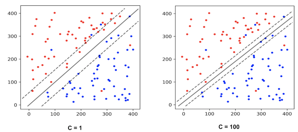] --- # Solution `$\qquad\qquad\qquad\qquad\qquad\qquad \hat{\beta}=\Sigma_{i=1}^{N} \hat{\alpha_{i}}y_{i}x_{i}$`.foot[1] - `$\hat{\beta}$` depends only on the Support vector points. - Predicted Class = `$Sign[x^{T}\beta + \beta_{0}]$` = `$Sign[\Sigma_{i=1}^{N} \hat{\alpha_{i}}y_{i}x_{i} x^{T} + \beta_{0}]$` - We don't even need `$\beta$` to get predictions. We just need `$\alpha_{i}$` for every support vector. .footnote[ [1] Elements of Statistical Learning, p 420-421 ] -- `$\qquad\qquad\qquad\qquad max L_{D} = \Sigma_{i=1}^{N}\alpha_{i} - \frac{1}{2}\Sigma_{i=1}^{N}\Sigma_{\hat{i}=1}^{N}\alpha_{i}\alpha_{\hat{i}}y_{i}y_{\hat{i}}x^{T}_{i}x_{\hat{i}} $` - `$\alpha$` values depend only on dot product between pairs of training datasets - Predictions depend only on dot product between support vectors and new data point - Dot products are central to SVM --- # Non linear separation? <br><br> .center.image-40[] ### Linear classifier doesn't look like a good option. -- Project data to higher dimensions, and classify there! .center.image-40[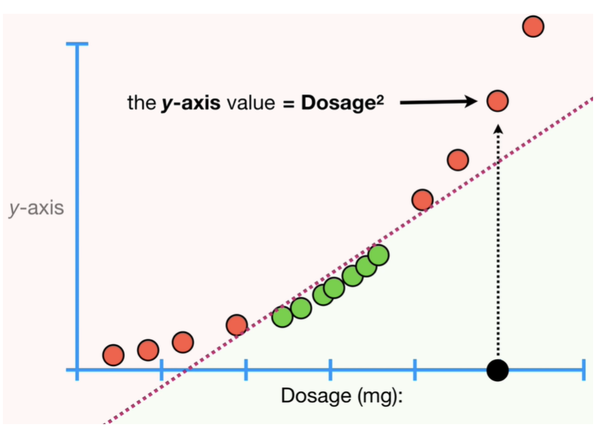] Can go to more dimensions as well. .footnote[https://www.andreaperlato.com/theorypost/introduction-to-support-vector-machine/] --- # Kernels - `$[x, x^{2}]$` is our new projection space - We need dot products only. So we want `$x_{1}x_{2} + x_{1}^{2}x_{2}^{2}$` - Define `$K(x_{1}, x_{2}) = (x_{1}x_{2} + r)^{d}$` - For `$r=\frac{1}{2}$` and `$d=2$`, `$K(x_{1}, x_{2})$` becomes `$x_{1}x_{2} + x_{1}^{2}x_{2}^{2} + \frac{1}{4}$`, or dot product between `$(x_{1}, x_{1}^{2}, \frac{1}{2})$` and `$(x_{2}, x_{2}^{2}, \frac{1}{2})$` - The function `$K(x_{1}, x_{2})$` gets us all information without projecting into higher dimensions - Any function K can act as a kernel as long as it satisfies following property: `$K(x_{1}, x_{2}) = < f(x_{1}), f(x_{2}) > $` - Above Kernel is called as Polynomial Kernel. `$r$` and `$d$` are hyperparameters - And this is called **Kernel Trick!!!** --- # RBF Kernel - What if we want to expand to infinite dimensions? i.e., `$x, x^{2}, x^{3}, x^{4}, .... $` -- - `$K(x_{1}, x_{2}) = e^{-\gamma ||x_{1} - x_{2}||^{2}}$` -- - From Taylor series, `$e^{x} = 1 + x + \frac{x^{2}}{2!} + ... = \Sigma_{n=0}^{\infty} \frac{x^{n}}{n!}$` -- - Let `$\gamma = \frac{1}{2}$` `$\qquad e^{-\frac{1}{2} ||x_{1} - x_{2}||^{2}} = e^{\frac{-1}{2} (x_{1}^{2} + x_{2}^{2})} e^{< x_{1}, x_{2} >} $` `$\qquad e^{\frac{-1}{2} (x_{1}^{2} + x_{2}^{2})} (1 + x_{1}x_{2} + \frac{x_{1}^{2}x_{2}^{2}}{2!} + ....)$` `$\qquad e^{\frac{-1}{2} (x_{1}^{2} + x_{2}^{2})} < (1 , x_{1} , \frac{x_{1}^{2}}{\sqrt{2!}} ,....), (1 , x_{2} , \frac{x_{2}^{2}}{\sqrt{2!}}, ....) >$` Let `$e^{\frac{-x_{1}}{2}} = s_{1}, e^{\frac{-x_{2}}{2}} = s_{2}$` `$\qquad < (s_{1} , s_{1}x_{1} , s_{1}\frac{x_{1}^{2}}{\sqrt{2!}} ,....), (s_{2} , s_{2}x_{2} , s_{2}\frac{x_{2}^{2}}{\sqrt{2!}}, ....) >$` - Therefore, RBF Kernel summarizes dot-product in infinite dimensions --- # Example svm_lin = SVC(kernel="linear") svm_lin.fit(iris_data.iloc[:, 0:2], iris_data["Y"]) svm_rbf = SVC(kernel="rbf", gamma=100) svm_rbf.fit(iris_data.iloc[:, 0:2], iris_data["Y"]) .center.image-60[] -- careful not to overfit. Use Cross-validation! --- # SVM Overview - _Maximum Margin Classifier_: Creates a decision boundary such that it separates the classes with as high margin as possible -- - _Support Vectors_: Data points that touch the margin. Other points far away from margin have no influence on decision boundary -- - _Support Vector Classifier_: When the classes are not perfectly separable, allows scope to have some errors -- - _Support Vector Machines_: Uses high dimension projections to identify non-linear boundaries -- - _Kernel Trick_: Gets same effect of high-dimension projections, without actually making the projections --- # SVM Overview (Contd. ) ### Pros: - Very useful when clear separations exist, even in non-linear spaces - Works well in case of large no:of features (high dimensional data). Works even if features are more than data points - Memory efficient as it needs to remember only the support vectors -- ### Cons: - Doesn't scale very well because of high training time - Doesn't give probabilities like Logistic Regression (expensive work-around) - Doesn't work well if there's lot of class overlap - Model gets heavier if features are high as more data points become support vectors --- layout: false class: center, middle # Decision Trees --- # Decision Trees - You want to send a marketing campaign about a new beauty product. How will you select your target customers? - _age_ + 100 * _isFemale_ `$\geq$` 120 - _age_ `$\geq$` 20 and _isFemale_ Which looks better? --- # Decision Trees Another Example .center.image-40[] --- # Iris Dataset .center.image-90[] - Root Nodes, Decision Nodes, Leaf Nodes - Tree Depth - Each leaf node denotes a category --- # Entropy How do we split a node? .center.image-40[] -- - Entropy: A metric for _randomness_. `$\qquad\qquad\qquad\qquad\qquad\qquad -\Sigma_{k=1}^{K}\hat{p_{k}}log(\hat{p_{k}})$` - At root node (50, 50, 50): `$- (\frac{1}{3}log_{2}\frac{1}{3} + \frac{1}{3}log_{2}\frac{1}{3} + \frac{1}{3}log_{2}\frac{1}{3}) = -log_{2}\frac{1}{3} = 1.585$` - At next (right) node (0, 50, 50): `$- (0log_{2}0 + \frac{1}{2}log_{2}\frac{1}{2} + \frac{1}{2}log_{2}\frac{1}{2}) = -log_{2}\frac{1}{2} = 1$` --- # Information Gain - Entropy at node N = `$H$` - Split causes two child nodes with entropy `$h_{1}$` and `$h_{2}$` and data points `$m_{1}$` and `$m_{2}$`. - `$p_{1} = \frac{m_{1}}{m_{1} + m_{2}}, p_{2} = \frac{m_{2}}{m_{1} + m_{2}}$` - Information Gain = `$H - (p_{1}h_{1} + p_{2}h_{2})$` -- - Choose the feature and split point based on largest information gain -- - For categorical features, each value is tried -- - For numerical features, deciles are used typically -- ### Gini Index: Similar to Entropy, simpler to calculate. `$\qquad\qquad\qquad\qquad\qquad\qquad \Sigma_{k=1}^{K}\hat{p_{k}}(1 - \hat{p_{k}})$` Produces almost identical results as entropy. More commonly used in practice. --- # Optimal tree - Continue growing forever and prune (trim) it -- - Limit based on max depth -- - Limit based on min no:of samples in a child node -- - Limit no:of features to check -- - Limit no:of maximum leaf nodes --- # Decision Boundary clf = DecisionTreeClassifier(max_depth=3, criterion="entropy") clf.fit(iris_data.iloc[:, 2:4], iris_data["Type"]) .center.image-50[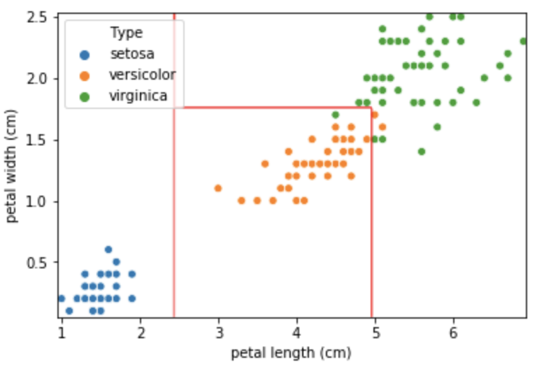] Non-linear boundaries, but piece-wise linear --- # Decision Trees Overview ### Pros: - Very intuitive, easy to understand, interpret, and communicate - Works well for multi-class problems too, without needing multiple models - Works well with categorical features w/o one-hot encoding/dummy variables etc - Feature selection happens automatically. If a feature is not important, it is not used -- ### Cons: - Tree building is done greedily, with a top-down approach. If data changes a little bit, can give a completely different model - Meaning, it has high variance i.e., poor performance on unseen data -- Solution? --- class: center, middle # Random Forests --- # Random Forests - A decision tree has high variance because small change in data can result in a very different tree. -- - Build _hundreds_ of trees (and take voting from them)!!! .center.image-90[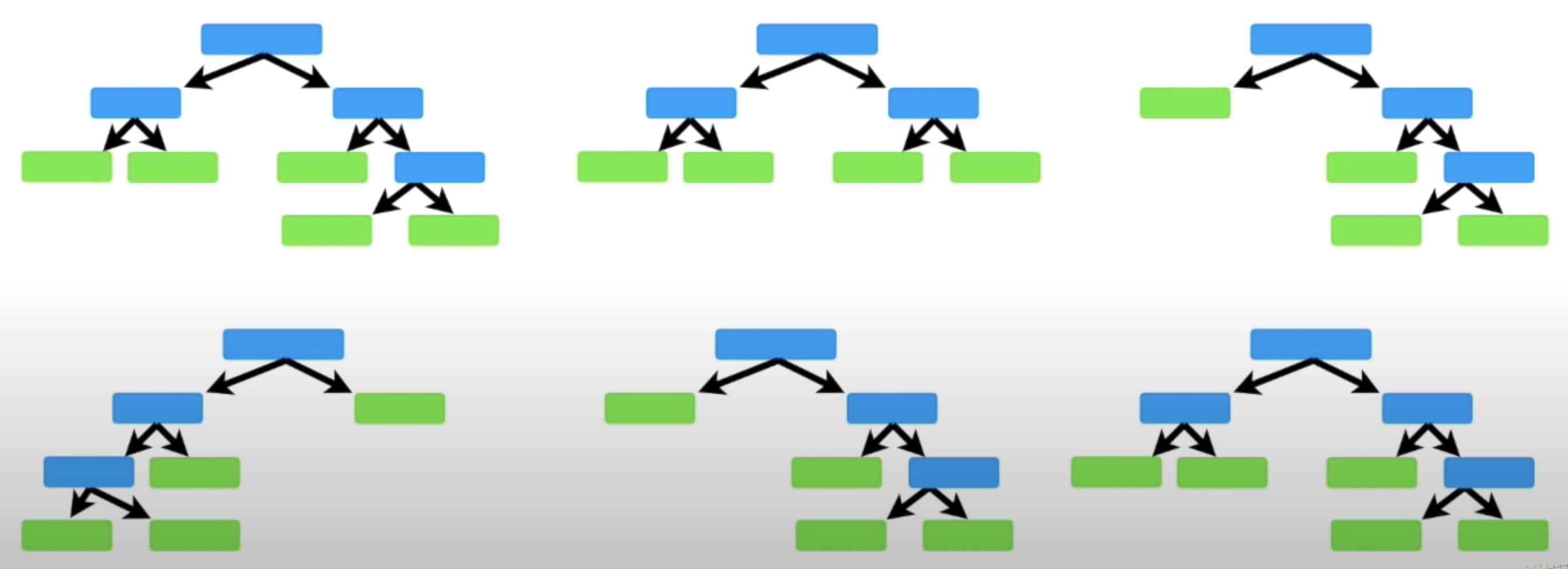] -- - All trees use same input data --- # Bootstrapping - Treat original data as a _source data_. Create new data set, which looks similar to existing data set - Sample with substitution (i.e., same data point can be picked again) - Build a data set as large as original data set. Some samples get represented multiple times. Some gets no representation. These points are called out-of-bag data - Randomly select some of the features from original data set - Build a tree - Repeat _n_ times - Each tree learns from different features, and different data points - Accuracy on the out-of-bag (oob) data can be used as a cross-validation score in some cases. No extra CV steps required - _Aggregate_ from the tree predictions - Bagging: **B**ootstrap the data and **agg**regate the results. --- # Decision Boundary rf = RandomForestClassifier(n_estimators=50) rf.fit(iris_data.iloc[:, 2:4], iris_data["Type"]) .center.image-50[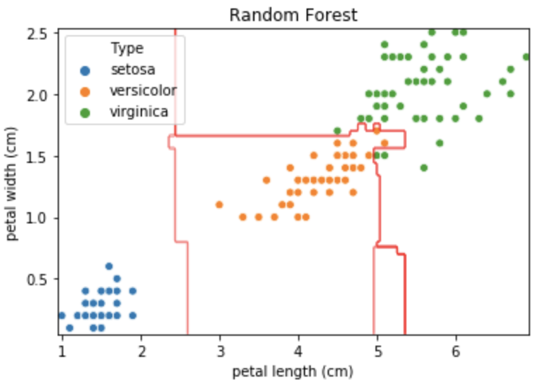] --- # Random Forest Overview ### Pros: - Does not overfit - Inherits benefits of Decision Trees w.r.t. categorical variables handling, and multi-class predictions ### Cons: - Loses the interpretability of Decision Trees - Doesn't work well if the decision boundaries are not axis aligned (ex: diagonal boundary) - Can't learn higher order representations - Doesn't work well with sparse data --- class: center, middle # Thank You